Facebook
 Google
 GitHub
 Linkedin
Hi MrAl!Hello again,
Hey that's pretty good. You got the transfer function right although you went through a lot of trouble to do that you could have used just Algebra, but you did get it right and that's great.
To design a filter first you have to know the application, and then you have to know how sharp you want the response to be. When you change the ratio of L/C (or C/L) you get either sharper or less sharp of a response and that has a large effect on your application. Because you also have R in series with L that means the response will be less sharp because of that also.
What you could do is look at some known filter types and their responses, or just plot some responses yourself with different L and C. You will start to get an idea how this works. You may be able to work from the ratios of L/C and L/C^2 and with the rest of the coefficients being just gains you can get an idea of the shape of the response from that and decide what ratio of L/C you want.
I guess we can look at a few different ways to do this if you like.
You can also probably use a curve fitting technique where you define two or three points on the response curve you want to use as reference points.
Thank you for your support.
I already said the application. This filter will be used to filter the input signal of the ADC and output of the DAC.
You asked me to derive the transfer function. Eventually, Done!. Ok. How can I plot the response from this transfer function?.
How to design the R, L, and C values?. These values will be used to design a filter that attenuate the signal above 100kHz.
S=jw, w=2*pi*f, and j2=-1. After substitution of these values, the final Transfer Function is derived and attached below. Please have a look and tell me how to plot the response from the below transfer function.
Attachments
-
36 KB Views: 15
Last edited: