Can you help me to understand Op Amps?

WBahn

Joined Mar 31, 2012
33,075
About the curve on a graph, If I just make 3 points, at 0v, 0.5v and 1v then I draw a line between them, won't be smooth and not accurate either, an oscilloscope makes a smooth curve (or almost) because of its refresh rate, right?
Depends on the type of scope. An analog scope has an electron beam that traces out a continuous trace on the screen as the signals cause it to deflect. A digital scope samples the input signal periodically and then generates a displayed waveform. There are several ways to do this. Most of the time, the samples are so close together that, to the human eye, they appear like a continuous trace. But, under certain conditions, you can definitely see the individual sample points.
 
I'm going to post 2 pictures, 1 of open loop and another of feedback resistor.
Coming late to this one, but please stop drawing lines through the middle of the op amp triangle - it's meaningless and confusing. As already stated, the gain of an op amp is very high so for most practical purposes you can assume that the amp will always do it's best to make the positive and negative inputs (nearly) equal to each other. If you force them to be different the output will swing (close) to the rail - positive rail if positive input is bigger than negative input or vice versa. If a feedback resistor can modify one of the input voltages as the output makes its way to the rail so the inputs become equal the amp is in its happy place. That's pretty much all there is to it.
 

MrChips

Joined Oct 2, 2009
35,022
About the curve on a graph, If I just make 3 points, at 0v, 0.5v and 1v then I draw a line between them, won't be smooth and not accurate...
You cannot do that, and here is the reason why you cannot do that.

Each data point is a pair of two parameters, voltage and time.
You can pick three voltage points, 0V, 0.5V, 1V, but you don't know the time it takes to reach those voltages.

You can pick three points in time, 0s, 1s, 2s, but you don't know the voltage attained at those times.

What we do know from experiments and by simple mathematical analysis is that change of current and voltage in this simple RC circuit does not follow a simple straight line, i.e. the rate of change is not constant. Hence any two points will be gross approximations of the behavior of the circuit, unless...

....unless we make our incremental steps so small that for all intents and purposes we can assume that the rate of change is constant.

Charge Q = Current I x Time t
Q = I x t

If we can assume that I is constant, then we can calculate Q over any length of time t.
Since we know that I is not constant, we need to make time t is small as possible so that any slight change in I will not adversely affect the accuracy of our analysis. We change t to dt, where dt represents a small increment in time.

Q = I x dt

Since this represents the additional charge added to the capacitor during the time dt, we should write this as,

dQ = I x dt

The point here is, if dt is too long (in time, hence few data points) we lose accuracy in our analysis.
In theory, we want dt to be infinitesimally short (hence infinite data points).
In practice, we only need to make dt short enough to give us accurate results. Ten to twenty data points in our area of interest is "good enough" to give us an accurate trend of what the circuit is doing. Three data points do not cut it.

(Application of the branch of mathematics called calculus uses infinitesimally small steps and therefore can give us exact mathematical solutions to problems of this nature.)
 

MrChips

Joined Oct 2, 2009
35,022
Ok. Let's say we are too lazy or don't have the time to calculate 10-20 data points.
We can put this into a spreadsheet program and get the computer to calculate the data set for us.

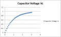
This is how I generated this Vc vs t curve.

1687872985955.png

If we have access to an oscilloscope, we can create this experimentally.
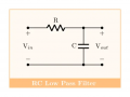
We simply replace the step voltage Vin with a square wave input signal.

1687873117719.png

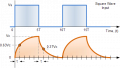
And presto, the oscilloscope at Vout will show us the capacitor charging and discharging cycles.


1687873139893.png
 

BobTPH

Joined Jun 5, 2013
11,616
Calculus is the branch of mathematics that allows us to get exact solutions for problems like this one, where things are changing continuously. The calculus solution is exact and what happens in the real world, unlike the approximations being done in this thread.
 

MrAl

Joined Jun 17, 2014
13,765
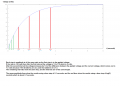
Friend do you mean something like the following image?View attachment 297158


Amplitude, peaks, thanks friend, let's say the first half cycle is positive, when the second half hits(negative), the positive charge in the cap will be discharged towards the signal(Vin)?

In a PWM, the time that the signal is High(ON or 1) is known as "Width", and + the Low time is known as "Period", or Period could be also the time from one High to the next High, is that right?
Hello again,

Yes for both.

When we look at a capacitor charging through a resistor that is fed by a constant DC source, we see that exponential curve (see attachment).
The basic formula is Vc=Vs*(1-e^(-t/RC)).

There is a little 'secret' here too that would lead to several exact values for the capacitor voltage. I will use an RC time constant R*C=1 for these illustrations.
If you take the same time step each time, the voltage changes by the same ratio as the ratio of the first step is to the applied voltage.
The red lines show what happens if you want to see steps in amplitude of 1/2 of the applied voltage minus the current voltage. First we see 5v because 10 minus 0 is 10 and times that 1/2 comes out to 5 volts. The next step is 10 volts (applied voltage) minus 5 volts (the current or last voltage calculated) divided by 2 (which is 5/2=2.5) and added to the previous voltage which was 5, and the total is 7.5 volts. The next step would be (10-7.5)/2=1.25v, and that added to 7.5v is 8.75 volts. These voltage levels are not approximate they are exact, but the catch is you have to move in time steps of exactly ln(2) which is the natural log of 2 which is about 0.693, and for the graph i approximated that to 0.7 to make it simpler to think about.

The green lines are interesting because when we take time steps of 0.1 seconds we get some approximations starting with 1v, then 2v, then 3v, etc., until we get close to 10v. So at 0.1 seconds we see about 1v, then at 0.2 seconds we see about 2v, and at 0.3 seconds about 3v. The actual exact changes are a little less that 1v though around 0.95 volts, but it's easier to think about using time intervals of 0.1 seconds and voltage steps of 1 volt each.
Note that if the applied voltage was just 1.00 volts, then the first voltage step for t=0.1 seconds would be 0.1 volts, so they are approximately the same. That means that when we normalize the voltage to 1.000 volts we get time steps that approximately match the voltage steps, and we can multiply the actual applied voltage by these normalized voltage steps to get close to the actual cap voltage in the application. For example, with 10v applied we see 0.1*10=1v, and if we had 20v applied we would see 0.1*20=2v per step, and of course with 100v applied we would see 0.1*100=10 volts for the first step, 20 volts for the second step, etc.

Ok, so i hope i complicated this enough for you now (ha ha) but this is pretty interesting i think, especially the 0.1 time step to 0.1 voltage step coincidence. We can also do the same with the RC time constant, so we have a template for calculating the charging of a capacitor with a series resistor and fed by a constant DC voltage and with no initial voltage. If there is an initial voltage we start with that, so its the same just the values will be different then. For example, if the initial voltage was 2v the first time step of 0.1 would produce a voltage of 3v.
The RC time constant spreads the curve out over time, so with RC=2 the time steps would be twice what they are in the illustrations. Thus this template could allow us to calculate the approximate voltage of any RC network fed by a constant DC source.
 

Attachments

Last edited:

MrAl

Joined Jun 17, 2014
13,765
Or you can use the exact formula as stated at the top of the previous post. The one derived by calculus.
Hi,

Ya think? (ha ha)

When we work with this stuff sometimes we look for approximations that allow us to quickly estimate the way something will perform. When we find something that correlates easily it not only allows this kind of estimate it also seems rather interesting that it worked out the way it did. Sometimes this helps to understand the basic properties of the circuit also which is always nice because then we end up with an intuitive understanding which helps remember how to do it also.
 

WBahn

Joined Mar 31, 2012
33,075
Or you can use the exact formula as stated at the top of the previous post. The one derived by calculus.
But if the TS doesn't understand calculus (they haven't answered my query about their math background), then this amounts to telling someone that asked, "what's the reason it doesn't look like a straight line?" that there's no need for them to try to understand the reason since here's an exact equation we are giving you that you can use.
 

MisterBill2

Joined Jan 23, 2018
28,027
Typical component tolerances and variations often render results that do not exactly match the calculated values. This can be a source of frustration for those who faithfully use the tedious formulas. ( The ones with log-exponents, as I recall.)
 
Top