Facebook
 Google
 GitHub
 Linkedin
Hi,
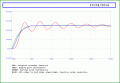
I've done a search & found a few references for '2nd order system approximation'. The issue I'm having is that none are for 4th order to 2nd, & the one that's closest shows how to transform a 5th to 2nd but the transfer function is much simpler.
I've done a search & found a few references for '2nd order system approximation'. The issue I'm having is that none are for 4th order to 2nd, & the one that's closest shows how to transform a 5th to 2nd but the transfer function is much simpler.
- Should it be the 'G(s) open-loop' that gets transformed from 4th to 2nd?
- Or should it be 'G(s) closed-loop' that gets transformed from 4th to 2nd?
- Link to G(s) open-loop: https://app.box.com/s/kh9dw3cpszaubioa44ia
- Link to G(s) closed-loop: https://app.box.com/s/28lg4l9ojm6xzau7r5ud
- Any instruction/help that could be offered would be really appreciated as I'm 100% stuck at this bit...