Facebook
 Google
 GitHub
 Linkedin
I'm trying to plot a cycloid curve, with a curve inside it and another one outside it, such that the inner curve and outer curve are equidistant along their entire length and the original curve lies between them.
Here is what I mean. I got the inner and outer curves in this picture by using a spline tool in CAD. I do not want to use a spline. I want to use an equation.

I've tried every single modification to the original equation that I can think of, and I've resorted to just embarrassing randomness. I've been at this for many hours and I'm wielding mathematics like a monkey with a machine gun at this point. Figured it was time to ask for help.
Here is what I mean. I got the inner and outer curves in this picture by using a spline tool in CAD. I do not want to use a spline. I want to use an equation.
I've tried every single modification to the original equation that I can think of, and I've resorted to just embarrassing randomness. I've been at this for many hours and I'm wielding mathematics like a monkey with a machine gun at this point. Figured it was time to ask for help.