Facebook
 Google
 GitHub
 Linkedin
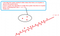
I am using least square method to find linear equation but getting some problems below.
Is there any idea for this?
Thank you.

Is there any idea for this?
Thank you.
Attachments
-
 15.4 KB Views: 350