Facebook
 Google
 GitHub
 Linkedin
The problem isn't that the simulation ended before 180 ms. The problem is that the period of integration is not an integral number of cycles (or at least half cycles). At 60 Hz, 180 ms is 10.8 cycles, so it would be hard, though not impossible, to get a valid result by averaging over 180 ms.Hi,
I did not try this yet, but why does your plot look like it ends before 180ms yet the calculation period looks like it is 180ms.
That could be why you got 81w instead of closer to 88w. If you fix that I would bet you get much closer to 88w.
The period of a 60 Hz waveform is (1/60)s so 180 ms is 10.8 cycles.
The power after the waveform stops does not go to zero, but is rather about midway between 0 W and 30 W. A glance at the current source parameters shows that it is specified to only produce ten cycles. After that, it stays at the DC value of 2 A which, through a 4 Ω load is 16 W, which tracks very nicely.
So the expected average over 180 ms would be the 88 W over the first 166.7 ms and 16 W over the remaining 13.3 ms, would would yield an average of 82.68 W. The displayed result of 81.57 W differs from this by just 1.3%. Looking at the waveform, the sampling artifacts are readily apparent and probably explain the minor discrepancy. The integration control parameters might also play a role.