Facebook
 Google
 GitHub
 Linkedin
It seems to me, and I'm looking for where I might have flawed thinking, that 2 sine waves, separated by 120
degrees [this has to do with 3 phase power] and summed [like when converting from 'Y' to 'Delta'] produce a
sine wave with sqrt(3) times the amplitude of either of it's contituent parts, but when doing the same for pulses
the resultant is twice as large as either constituent part. It seems the harmonics traveling with the pulse [as
in Gibbbs phenomena] add 15% to the amplitude of the resultant over what it would be with just sine waves.
Am I understanding this correctly? To check this I made an 'R' file I've attached below. I ran out of a line
to put the program on before I got to add in all the harmonics I was interested in, but the results seem to
follow unless I'm doing something wrong.
% 'R' program start
par(mfrow = c(2, 3))
curve(sin(x), from = 0, to = 7, n = 1001)
curve(sin(x-(2*pi/3)), from = 0, to = 7, n = 1001)
curve(sin(x) - sin(x-(2*pi/3)), from = 0, to = 7, n = 1001)
curve(1.1547*(sin(x)+sin(3*x)/3), from = 0, to = 7, n = 1001)
curve(1.1547*(sin(x-(2*pi/3))+sin(3*(x-(2*pi/3)))/3), from = 0, to = 7, n = 1001)
curve(1.1547*(sin(x)+sin(3*x)/3-(sin(x-(2*pi/3))+sin(3*(x-(2*pi/3)))/3)), from = 0, to = 7, n = 1001)
par(mfrow = c(1, 1))
% 'R' program end
Thanks much for checking my work
WarrenR
degrees [this has to do with 3 phase power] and summed [like when converting from 'Y' to 'Delta'] produce a
sine wave with sqrt(3) times the amplitude of either of it's contituent parts, but when doing the same for pulses
the resultant is twice as large as either constituent part. It seems the harmonics traveling with the pulse [as
in Gibbbs phenomena] add 15% to the amplitude of the resultant over what it would be with just sine waves.
Am I understanding this correctly? To check this I made an 'R' file I've attached below. I ran out of a line
to put the program on before I got to add in all the harmonics I was interested in, but the results seem to
follow unless I'm doing something wrong.
% 'R' program start
par(mfrow = c(2, 3))
curve(sin(x), from = 0, to = 7, n = 1001)
curve(sin(x-(2*pi/3)), from = 0, to = 7, n = 1001)
curve(sin(x) - sin(x-(2*pi/3)), from = 0, to = 7, n = 1001)
curve(1.1547*(sin(x)+sin(3*x)/3), from = 0, to = 7, n = 1001)
curve(1.1547*(sin(x-(2*pi/3))+sin(3*(x-(2*pi/3)))/3), from = 0, to = 7, n = 1001)
curve(1.1547*(sin(x)+sin(3*x)/3-(sin(x-(2*pi/3))+sin(3*(x-(2*pi/3)))/3)), from = 0, to = 7, n = 1001)
par(mfrow = c(1, 1))
% 'R' program end
Thanks much for checking my work
WarrenR