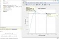
I started studying classical control at 2 months and my teacher spent an exercise to make a PI compensator of the open-loop transfer function attached, so that it has the following specifications. Ts2%= 2s; overshoot = 16% and overshoot at = 0.9s and Ess = 0
But how can I obtain the damping and natural frequency of a higher order system from the given specifications so that I can calculate the new dominant poles for it then I can calculate the zero of the compensator so that it has the necessary angular contribution?

obs .: initially I had followed the steps as if it were a second order system, but as you can predict the specifications were not reached, I even managed to find a good approximation with the help of Matlab but as this was not the purpose of the exercises I could not present in this way, the objective was to find the answers and prove mathematically the result, the aid of Matlab was at most to plot the root locus

 

I forgot to say it was for the step answer. any data that someone thinks I have omitted, please ask

 

Hi,

Are you trying to find a second order approximation from a third order system?
There are various ways to go about doing this, but it would be best if you show a block diagram of your final system even if you cant write in the gains for the feedback yet.

Some things in design are very straightforward, and some things are in the grey area where there are various ways to handle it. If you have been taught something about this in the past, then you should default to that way, but we can take a look at your system and see what we can find out.

 

Hello, i have studied again and I think that approximation is not necessary since the transfer function is of the second degree as indicated above and has a negative unitary feedback; I think I made a mess because of the addition of the compensator will add a pole at the origin and a zero. But I came across that the design of the compensator continues to give the wrong constant (I put only the proportional constant, since the integral constant can be found at zero of the compensator).

 

Hello, i have studied again and I think that approximation is not necessary since the transfer function is of the second degree as indicated above and has a negative unitary feedback; I think I made a mess because of the addition of the compensator will add a pole at the origin and a zero. But I came across that the design of the compensator continues to give the wrong constant (I put only the proportional constant, since the integral constant can be found at zero of the compensator).

Hi,

I'd like to help more but i prefer to see your block diagram first. That should not be hard to draw.

 

my teacher did not give the diagram he just described it as I had previously described; he just said the open loop transfer function and it says that the system has a negative feedback unit and that is to have the parameters quoted earlier for a unit step input

 

my teacher did not give the diagram he just described it as I had previously described; he just said the open loop transfer function and it says that the system has a negative feedback unit and that is to have the parameters quoted earlier for a unit step input

Hello,

So then you should be able to draw it yourself then.
It's up to you if you want to draw it or not but it would be better if you did.
If you cant draw it then you dont know how it connects and that's a first step to solving this.

 

this I understood from the problem, the PI compensator cascaded with the system transfer function.

 

Hello again,

If you use the integrator in the feedback then the transfer function is third order, but yes if you do not use that then you end up with for example:
(100*K)/(100*K+s^2+5*s+6)

and that's second order.

So if your procedure is to do it that way, then what went wrong?
Perhaps you should quote your entire procedure.

 

as the latex tutorial of the site does not seem to work with me I wrote the steps I followed in the PDF, I think I missed the angular contribution or the module condition.

 

as the latex tutorial of the site does not seem to work with me I wrote the steps I followed in the PDF, I think I missed the angular contribution or the module condition.

Hello,

Did you try graphing your solution?
It looks like it might be close, but i am not sure i understand your specs exactly.

Are you saying you have to have settling to 2 percent within 2 seconds, and overshoot max of 16 percent?
And your peak has to be at 0.9 seconds?
Is all this correct or no?

Graph (first pic Response1.gif) of your current solution, is it close to what you want or not?
Second graph Response2.gif (modified params Kp and Ki), is that closer to what you want or no?

 

yes, the settling time to 2 percent is 2 seconds, overshoot of 16 percent and peak at 0.9 seconds.
It's little strange cause when i command the step response to function already with the compensation the overshoot is about 7%, settling time is 2.32 seconds and peak at 0.96 seconds. i think it's like your "response-1". but the correct response is like your "response-2"

 

yes, the settling time to 2 percent is 2 seconds, overshoot of 16 percent and peak at 0.9 seconds.
It's little strange cause when i command the step response to function already with the compensation the overshoot is about 7%, settling time is 2.32 seconds and peak at 0.96 seconds. i think it's like your "response-1". but the correct response is like your "response-2"

Hi,

If you used some kind of software to plot the graph then it should be similar to "response-1" because that is the response using your transfer function and compensator parameters. I was hoping "response-2" came out to be nearly what you wanted so i understand your problem better.

In order to find out what is going on here i'd have to see your entire procedure not just some equations. I'll also see what else i can find around here and on line. I have a feeling it could be because the dominate pole is not dominate enough and the other one contributes more than might be expected, but that's just a guess right now. The procedure might be assuming the dominate pole is much more significant but i'd have to see the theory on the procedure being used.

The reason i asked about going third order to second order was because the response is third order and if it was approximated by a second order it could very well come out being very useful to predict the third order response. The technique is a little involved though.

LATER:
Ok it appears that you are using a somewhat standard method for 2nd order systems.

Yes, using the expression (for one example):
Ts=4/(wn*zeta)

is for a second order system where we assume that represents the dominant response. If it is not significantly dominant, then that's not as good of an expression to use. To get a better choice we would have to use an approximation to the third order system by a second order system, and that would come from a procedure made for that. We would end up with a second order system that mimics the third order system good enough to use that second order dominate technique.

I dont know how good you need this to be though either. For example if you just change the constants a little you can do a numerical tracking where when you change one constant by a small amount the peak changes by some amount, and you can use that info to pick a new constant. This is sort of trial and error though so i am not sure you want to default to that idea. The solution lies in plotting the time function and checking with some calculus if you want to be more exact.

 

how did you do the "response-2" ? with an approximation to the third order system by a second order system? I thought the approach was only made if the system function was of a higher order(in my case is second order), but are you saying that I need to take into account the compensator also to define whether the system is higher order or not?

 

Hello again,

Well, if we have a transfer function of order 3 then we have a transfer function of order 3, which means the unforced transfer function is of order 3, not of order 2. That means that whatever goes into that third order system (constants, etc.) usually has an effect on the output response with a certain input excitation (unit step), and since the third order system has a more complicated denominator than the second order system then the output is going to be more complicated in general, having effects from at least one extra constant and one extra power of the variable 's'.
So for example we have denominators:
a*s^3+b*s^2+c*s+d

versus:
A*s^2+B*s+C

so the third order system is dependent on more constants and powers of s. In short, it's a different transfer function.

Now if the 3rd order system has two dominant roots, then the 3rd order system might give almost the same output as a second order system where the two dominate roots are used to meke a second order system and that has ALMOST the same output as the third order system because that third root doesnt do much.
The problem is though that if the third order system does not have a dominate pair of roots, then all three roots have a play in the response, so simply dropping one out results in a 2nd order response that does not closely match the 3rd order response. In that case it becomes necessary to convert the third order system to a second order system using a more accurate conversion technique. In the more advanced technique we hope to see the resulting second order system emulate the third order system more accurately. It may simplify the parameter selection procedure or make it harder, but it should result in a more accurate selection.

Although a third order system is more difficult than a second order system, it's not impossible, so another idea is to use a numerical technique, or try to convert the response into a time response and look at certain features. To convert to a time response we find the Inverse Laplace Transform and that gives us something to work with. To use the numerical technique, we would use a second or third order ODE solver technique. In either case though we have some complication because we have two 'constants' we have to find, which are really variables in this problem, so we have a two dimensional solver problem which is a lot more complicated than a one dimensional solver problem.
When i found the second response i had shown previously, i used the time domain idea and simply looked for a time response that wss somewhat what i thought you might be looking for. Thus, i took your two values and as trial values increased them both by something like 0.1 and i got a response that looked like that which is somewhat close to what you were probably looking for.

But let's digress for a minute here. Maybe you just made a mistake somewhere in the math?
You used a second order system to find your two values which i call Kp and Ki where Kp is the proportional constant and Ki is the integral constant. If you can show me which second order system you used to start with, i can check your results better i think.
For example, did you just use the original G=100/(s+2)*1/(s+3) which of course is G=100/((s+2)*(s+3)) which is:
G=100/(s^2+5*s+6)

and work with that, or did you place it into the closed system and come up with:
T=G/(G+1)=100/(s^2+5*s+106)

and work with that instead?

This will allow me to follow your work better.

Lastly, you will note again that the transfer function for the system with the compensator in the forward path leads to a system with a denominator of third order, which is not the same system as any above and therefore we will expect a different output.

 

Hi again,

I took another look at this problem and it starts to look like this problem may be over specified or else we just have to be willing to accept some error in one of the specifications. I say this because we have three specifications:
1. Ts, the settling time to 2 percent or better (2 sec).
2. Tp, the time to the peak (0.9 sec).
3. PO, the percent over shoot (16 percent).

yet we only have two parameters to vary, Kp and Ki.
This usually does not work in general unless we get really lucky and the third spec just happens to fall into place once we get the other two.

Using an optimization method, we might look at six derivatives as we vary Kp and Ki:
dTs/dKp and dTs/dKi,
dTp/dKp and dTp/dKi,
dPO/dKp and dPO/dKi

and this will tell us the effect each variation of Kp and Ki has. We can then set up a table and decide which variation represent an improvement. That is, when the derivatives point in directions that are synonymous with an improvement of Ts, Tp and PO.
This is something like the method of steepest decent or similar.

Applying this method by hand and accepting some small errors in Kp and Ki, i can get two specs to come iinto near exactness but there's always one spec that doesnt quite make it to a very close approximation, although in the practical case it would still be considered good.
For the two i did last, i was able to get Ts and PO nearly exact, while Tp came in around 0.8 seconds which differs from the spec of 0.9 by about 12 percent.

In many 3rd order examples we see they always seem to have easily factored denominators. That's not the case here so that makes it more difficult. We can factor the denominator, but solving for Kp or Ki is then very difficult if not impossible unless we use a numerical method perhaps (didnt try this yet).
In still yet other 3rd order examples they are simply going after a response that is considered optimum by some integral standard. In that case they give the third order denominator and we are to adjust parameters to match that, so we are not after a certain wave shape then based on instantaneous values at certain times, but instead on an area.

A last thought for now is that maybe the original calculation was to be taken as adequate for the problem, being close enough anyway perhaps.

The following plot shows the time domain response found using this optimization method. It gets pretty close and so is probably good for the practical circuit.
The peak time is only slightly off, and the settling time is only off by about 1 percent.
The values for Ki and Kp are shown.
The controller form was:
Kp+Ki/s

Some levels and time values are conveniently shown as horizontal lines, and the peak time is shown as an impulse at t=0.9 seconds (black). The derivative is shown so we can pinpoint the peak time.

 

Hi,

Another simple view on the difference between the second order system and the third order system goes like this...

Suppose we have a 2nd order system with response as in the previous post (forget for a minute that is a solution to the current problem). The transfer function denominator would be such as:
s^2+a*s+b

Now just suppose that we wanted to, for some reason, filter that output with a low pass filter:
1/(s+c)

What would the transfer function look like? It would look exactly like the convolution of the 2nd order system with the low pass filter:
(A*s+B)/(s^2+a*s+b) * 1/(s+c)

so the denominator would be:
(s^2+a*s+b)*(s+c)

which is the third order system we are working with now.

Now we know a low pass filter decreases the higher harmonics, so we would expect to get a "smoother" output response. That means that the second order factor must have a damping ratio that is LESS than the second order system, because the peak wont go as high due to the low pass filter effect.

I might be able to post more about this later.

 

Hello, I was in month of exams so I was out of the discussion.
i speak with my teacher about this problem so he simulated the algorithm in matlab and had the conclusion that my answer was compatible with his idea (despite the incompatible answer with the desired parameters), but I said of the case that the compensator would cause the third degree function not to be as a good approximation of a function of the second degree so that we can use the standard formulation of the second degree function and he agreed.

I'm reading Ogata and I don't remember that optimization method you mentioned earlier, if you could describe it better I would appreciate it.

One more thing, my teacher said that the idea was as you said before, we could calculate two parameters and the third would be where we want.

 

Hello again,

Hello, I was in month of exams so I was out of the discussion.
i speak with my teacher about this problem so he simulated the algorithm in matlab and had the conclusion that my answer was compatible with his idea (despite the incompatible answer with the desired parameters), but I said of the case that the compensator would cause the third degree function not to be as a good approximation of a function of the second degree so that we can use the standard formulation of the second degree function and he agreed.

I'm reading Ogata and I don't remember that optimization method you mentioned earlier, if you could describe it better I would appreciate it.

One more thing, my teacher said that the idea was as you said before, we could calculate two parameters and the third would be where we want.

I am happy to hear you have more time now, and that you got to verify some of what we were talking about.

Did you ever use a method like steepest decent, or something like that?
If you did, that will help explain this.
I should mention though that i have not yet algorithmitized the procedure for this problem just yet, but you may want to do that. I might have a set of lines of code around somewhere though that might handle this.

The basic idea is to first realize that we only have two or three variables we have to work with. I think this had just two which makes it even simpler.
Having two variables Ki and Kp, we know that we want to find two that work good, even if not really super perfect, as long as they are close. That means that if these two Ki and Kp were to change the function orthogonally and we changed Ki the results would be exactly independent of the results we got from changing Kp. For the functions we will encounter however, it's unfortunate but we wont get this kind of variable independence, as some of the effects from each will be affected by the other as well. Now if we could rotate the problem space, we could align Ki and Kp (as other variables perhaps) to perturb the function orthogonally as would be ideal, then we would really have it made because each one would act on their own without interference from the other. That's the most advanced way to do this, but it takes a bit of programming to get to that point, so i will digress to the method where we leave them alone and just apply a steepest decent technique anyway and try to find a decent solution, even if it is not the absolute perfect one with extreme accuracy. The solution should be good in any case, or we try again.

Ok so the basic idea then is we start with the two variables Ki and Kp, and we know that if we were to change them we only have four choices:
[11] Ki+dKi, Kp+dKp
[10] Ki+dKi, Kp-dKp
[01] Ki-dKi, Kp+dKp
[00] Ki-dKi, Kp-dKp

although sometimes these choices are used also:
Ki+dKi, Kp
Ki-dKi, Kp
Ki, Kp+dKp
[00] Ki, Kp-dKp

I've enumerated the top four choices in binary to show that each 'bit' represents a sign of either plus or minus. Note that we change two variables at a time, unless we use the second set too which we'll skip for now and assume that the increment size can handle those choices by sheer size.

So the idea is simple. Start with a small but not super small increment for each variable, dKi and dKp. Calculate whatever it is you want to calculate with starting values for Ki and Kp, then calculate again with each of the four choices. Whatever produces the lowest error, adopt that value for the next calculation and reduce the increment for the respective variable by 1/2 (divide it by 2).
After several passes, the increment no longer produces a change in the error, and ideally you have the solution.

The function you will calculate will be the peak and the settling time so you have to calculate the square root of the sum of squares of the errors.

I guess we could look at ways to achieve all this, but see what you can make of it so far.

 

[note: had to fix some typos]

Hello again,

Here is an example of the output of such a procedure.
In this example, the variables are Ap and Ai which are just Kp and Ki multiplied by 100, so to get Kp and Ki just divide what is shown by 100.

The format for each section is:
[. .] which shows which vars were incremented or decremented, and a period means the var was not changed.
The next line is:
Time to peak, peak value, value at t=2 seconds, Ap,Ai
The third and final line is:
Error in time to peak, error in peak value, error in value at t=2 seconds compared to 2 percent, sum of squared errors.

Now if we look at just the sum of squared errors, we see that the lowest one is 0.000532 and normally the values for Ap and Ai just above that would be taken to be the next set to start with. However, we might have more concern for the time to peak value itself than the settling time for example. In that case we may wish to simply choose the group with the lowest time to peak value so we can try to get that spec better. The second group there looks better for that spec so we might try that Ap,Ai set instead for the next run.

I had sort of forgotten that i set the solution up in the form of three ODE's and then solved for everything numerically over a 5 second period. That was a little easier than doing the inverse transform over and over again.
The ODE set was this:
x1=E*Ai-Ai*X3,
x2=X1+E*Ap-(Ap+6)*X3,
x3=X2-X3*5

where E is the input step voltage and X3 is the output voltage.
Ap=Kp*100, Ai=Ki*100, and the other constants come from the transfer function also but dont have to be variables.
I used a 3rd order Taylor method to solve the ODE's numerically.
The program to do this was not put into a purely algorithmic form yet though. The next step would be to add another loop that automatically searches for the optimum value(s) desired. There will be a tradeoff anyway though.

Some caution has to be observed when using these kinds of methods though. For one, the algorithm could get stuck at a local minimum, and that makes it look like we've found the best solution when really it's not exactly so. It may be good enough though, or we simply do a brute force search which for two variables doesnt take that long. The other possibility is that we land on an absolute min, but the width is very small. In that case we have to evaluate the slopes in getting there to make sure that the solution will be practical (such as sensitivity analysis for example). A less optimum solution may be much more stable in the practical world when we have to deal with component value tolerances and stuff like that.
Also, as the number of variables increases it takes longer and longer to do the search, so it may start to become too long with some number of variables. For just two variables it is rather fast though.

In any case, it's worth doing at least one time it's interesting to see the results start to show up as better and better.

There are more advanced methods using matrixes but that involves either more programming or software that can do it already.