Facebook
 Google
 GitHub
 Linkedin
Not really homework : not for school grade
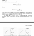
Please look at images : been trying for a while now to reproduce the images on Matlab ..
Perhaps Ts is missing the point..Is he?
Thanks
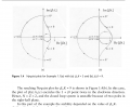
Please look at images : been trying for a while now to reproduce the images on Matlab ..
Perhaps Ts is missing the point..Is he?
Thanks
Attachments
-
 404.1 KB Views: 9
 -
 603.6 KB Views: 9