Why is it possible for a first order closed loop system to have a step response with an overshoot or become marginally stable?

 

Why would anybody consider a REAL first order control loop system to ever be stable? Every real system has some response delay, which equates exactly to a phase shift, and at some amount of gain at some frequency that combination will first cause overshoot, and then with more gain it will provide oscillation.

 

Research PID loop.
Max.

 

Research PID loop.
Max.

A PID loop is at least a third order feedback system. Proportional + Integral + Derivative. Of course the explanation of that does indeed demonstrate why a first order loop can overshoot and even oscillate.
I have observed that a bit of deadband can be useful to stabilize a loop, but I have not done the math to see if it is adding another "order" or not. I guess that it is close to the Integral function, but possibly not.

 

Hello,

The overall transfer function tells the story.
A transfer function that is 2nd order of above can have overshoot, but a first order can not.
That is looking at the complete transfer function of the system.
In a 2nd order system the damping factor tells us what the overshoot will be if there is one.

 

Hello,

The overall transfer function tells the story.
A transfer function that is 2nd order of above can have overshoot, but a first order can not.
That is looking at the complete transfer function of the system.
In a 2nd order system the damping factor tells us what the overshoot will be if there is one.

If we can define a contactor servo as a first order system, and if the servo does not have instant brakes and motor response, it will have some amount of overshoot. The exception is if it is run on a simulator where there is no inertia or delayed response.

 

If we can define a contactor servo as a first order system, and if the servo does not have instant brakes and motor response, it will have some amount of overshoot. The exception is if it is run on a simulator where there is no inertia or delayed response.

Hi,

It sounds like what you are talking about is an isolation of two systems calling one first order and ignoring the second and then stating that there is still overshoot. But if there exists an electro-mechanical system where the electronic part is first order that doesnt mean the transfer function of the system is first order. When we have both electronic and mechanical the two form one system and so the transfer function is from the electrical input to the mechanical output. Now if the entire system is first order there can be no overshoot (just look at any first order transfer function) but if it is second order (or higher) then there might be overshoot.
Examples of first order is a resistor in series with a cap, or a resistor in series with an inductor.
A motor by its very nature is always at least second order although the mechanical part may dominate the overall response.

 

Why would anybody consider a REAL first order control loop system to ever be stable? Every real system has some response delay, which equates exactly to a phase shift, and at some amount of gain at some frequency that combination will first cause overshoot, and then with more gain it will provide oscillation.

Why does the increase in gain and phase shift cause instabilty, oscillation.....

 

Why does the increase in gain and phase shift cause instabilty, oscillation.....

Hi,

It is just the nature of it. If you do a root locus plot you can see what gain starts to cause oscillation because the plot crosses the jw axis. In a root locus plot with the gain being the variable, we can see how the poles migrate and if they stay in the left half plane the system is stable but if they move into the right half plane for certain gains then those gains will produce either a constant oscillation or a rising exponential that eventually saturates the system. So the idea is to learn what the limit is on the gain in order to maintain a stable system.

 

Hi,

It is just the nature of it. If you do a root locus plot you can see what gain starts to cause oscillation because the plot crosses the jw axis. In a root locus plot with the gain being the variable, we can see how the poles migrate and if they stay in the left half plane the system is stable but if they move into the right half plane for certain gains then those gains will produce either a constant oscillation or a rising exponential that eventually saturates the system. So the idea is to learn what the limit is on the gain in order to maintain a stable system.

Is it possible to work out the transfer function of a closed loop system if you only know the open loop transfer function.

And input to the closed loop system

 

Why does the increase in gain and phase shift cause instabilty, oscillation.....

The non-math explanation is that when the phase shift becomes large enough to make whatever feedback add rather than subtract, things may be unstable, and when the loop gain becomes greater than the losses, the signal will continue to becoming larger, instead of fading away.

 

Is it possible to work out the transfer function of a closed loop system if you only know the open loop transfer function.

And input to the closed loop system

Hi,

Yes. It is G/(1+G*H) where G is the forward gain and H is the feedback gain and the feedback is negative. IF the feedback is positive then change that plus sign to a minus sign.
What are you trying to do here?

 

Hi thank you for your help. I want to determine the stability of the closed loop system using root locus as you mentioned I can use in a previous message. What would be the transfer function of the closed loop system I have attached. do I multiply the open loop transfer function with 2/1+2 (this is G/(1+G*H) assuming internal gain is 2)

 

Why is it possible for a first order closed loop system to have a step response with an overshoot or become marginally stable?

Sounds like a homework question. Is it? If so, we can move the thread to Homework Help where it will get the kind of attention it needs.

 

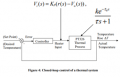
Hi thank you for your help. I want to determine the stability of the closed loop system using root locus as you mentioned I can use in a previous message. What would be the transfer function of the closed loop system I have attached. do I multiply the open loop transfer function with 2/1+2 (this is G/(1+G*H) assuming internal gain is 2)

Hi,

You first have to define the transfer function of every block in your block diagram.
Can you see that the feedback factor is just 1 because there is no gain in the feedback path?
It is actually -1 but we dont use the minus sign in the formula:
G/(1+G*H)

and so in that formula H=1.
But we need the blocks defined in order to know what G is.

 

https://eclass.upatras.gr/modules/document/file.php/EE817/PT326.pdf

Hi thank you again for your help

ive been reading the link that i have placed above and from what i understood i labbled the block diagram

ive used a formula, i found on the internet which is

T(S) = (GcGp)/(1+GcGp)

from the picture above i made Gc =kp

Gp =

therefore i got

T(S) = (kp)(k)(e^(-tds))/ts+1+(kp)(k)(e^(-tds)

How can i determine the stabilty of this closed loop transfer function if it is correct

 

Hello,

You need to make your expressions a little clearer especially by using parentheses when needed.
I think you mean this:
T(S) = kp*k(e^(-td*s))/(t*s+1+(kp*k)(e^(-td*s))

When there is no delay in the system we have functions like this:
k*(s+a)/(s^2+b*s+c)

and then we do a root locus procedure with k or kp varying. You can look that up and see what you can find.
However this system has a delay so i'll have to look up the best way to handle that.
Another way is to plot the transfer function using a Laplace voltage to voltage source using all the known values and making either k or kp vary. The system output can then be viewed and a decision made as to whether or not the system is stable enough. Note i am using the phrase "stable enough" because systems that are stable are not always acceptable because they still oscillate too much before damping.
Another possibility is to transform into the z domain and do a discrete analysis.
Also, note that systems with delays may have overshoot even though otherwise first order mainly because they are not true first order systems anymore.

Another way to handle the delay is to use a polynomial approximation. But if you want to do that, i would advise learning the root locus process on a non delayed system first. Once you master that, you will be in a better position to do the delayed system with delay approximation.

Anyway, for simulating what simulator do you use or can get to use?

 

Hello,

You need to make your expressions a little clearer especially by using parentheses when needed.
I think you mean this:
T(S) = kp*k(e^(-td*s))/(t*s+1+(kp*k)(e^(-td*s))

When there is no delay in the system we have functions like this:
k*(s+a)/(s^2+b*s+c)

and then we do a root locus procedure with k or kp varying. You can look that up and see what you can find.
However this system has a delay so i'll have to look up the best way to handle that.
Another way is to plot the transfer function using a Laplace voltage to voltage source using all the known values and making either k or kp vary. The system output can then be viewed and a decision made as to whether or not the system is stable enough. Note i am using the phrase "stable enough" because systems that are stable are not always acceptable because they still oscillate too much before damping.
Another possibility is to transform into the z domain and do a discrete analysis.
Also, note that systems with delays may have overshoot even though otherwise first order mainly because they are not true first order systems anymore.

Anyway, for simulating what simulator do you use or can get to use?

Hi,

i do not know what Laplace voltage to voltage source and z domain is. i only recently learnt root locus when you mentioned that this can be used. Im self teaching myself control systems with the help of this forum

how did you go from

T(S) = kp*k(e^(-td*s))/(t*s+1+(kp*k)(e^(-td*s))

to

k*(s+a)/(s^2+b*s+c)

I was reading that if a pole is on the right side of the graph it is unstable so how can i calcuate the poles. I cant find an example online which has a time constant in the transfer function

 

Hi,

i do not know what Laplace voltage to voltage source and z domain is. i only recently learnt root locus when you mentioned that this can be used. Im self teaching myself control systems with the help of this forum

how did you go from

T(S) = kp*k(e^(-td*s))/(t*s+1+(kp*k)(e^(-td*s))

to

k*(s+a)/(s^2+b*s+c)

I was reading that if a pole is on the right side of the graph it is unstable so how can i calcuate the poles. I cant find an example online which has a time constant in the transfer function

Hi again,

First i did not go from your transfer function to k*(s+a)/(s^2+b*s+c) even though we might try that route too at some point, possibly ending up with a more complicated equation though. But that was just an example of a more typical system that we wanted to study. In that form it really has nothing to do with this system at hand just yet.

I have long since converted my own knowledge of the root locus into an automated program some years back and that's what i use, so i will have to dig into my notes and find out the way to handle this.
The most intuitive way to view this is that you work with the transfer function to get it into a certain form and then try to find the complex roots repeatedly and plot them as you vary some parameter like kp. But in this system the time constant will play a big part in the relative stability in a way similar to how the coefficient of 's' affects the roots in a regular polynomial system because the coefficient contains the damping factor which affects the overshoot and settling time.
Give me some time to review my notes on this, but it would be worthwhile i think to look at a system with no delay and find the roots and see how they migrate s some parameter like the gain is varied.

[LATER]
Gee i found an example on the web like on the first try.
The first thing to do is form G*H where G is the open loop path and H is the feedback path.
The example was with G*H=K/(s*(s+3)).
The characteristic equation is 1+G*H=0
which here is 1+K/(s*(s+3))=0
or K+s^2+3*s=0
Now the roots start at K=0 and extend to K=inf. The idea is to
see if any of the roots move into the right half plane as K is varied which would mean the real part of the complex solutions becomes positive. If the roots start out on the left hand side and then for some K the real part become positive then the system is unstable starting with that value of K.
The solutions for this equation are rather simple so i'll state them here...
s1=-(sqrt(9-4*K)+3)/2
s2=(sqrt(9-4*K)-3)/2

and we can see that the solutions are real for K=0 to 9/4 and complex for K>9/4. But the real part is what tells us initially if the solutions migrate into the right hand plane.
The idea for the locus now is to plot several solutions and see how the solutions migrate and if any move into the right hand plane. See if this makes sense to you so far.

 

Hi again,

First i did not go from your transfer function to k*(s+a)/(s^2+b*s+c) even though we might try that route too at some point, possibly ending up with a more complicated equation though. But that was just an example of a more typical system that we wanted to study. In that form it really has nothing to do with this system at hand just yet.

I have long since converted my own knowledge of the root locus into an automated program some years back and that's what i use, so i will have to dig into my notes and find out the way to handle this.
The most intuitive way to view this is that you work with the transfer function to get it into a certain form and then try to find the complex roots repeatedly and plot them as you vary some parameter like kp. But in this system the time constant will play a big part in the relative stability in a way similar to how the coefficient of 's' affects the roots in a regular polynomial system because the coefficient contains the damping factor which affects the overshoot and settling time.
Give me some time to review my notes on this, but it would be worthwhile i think to look at a system with no delay and find the roots and see how they migrate s some parameter like the gain is varied.

[LATER]
Gee i found an example on the web like on the first try.
The first thing to do is form G*H where G is the open loop path and H is the feedback path.
The example was with G*H=K/(s*(s+3)).
The characteristic equation is 1+G*H=0
which here is 1+K/(s*(s+3))=0
or K+s^2+3*s=0
Now the roots start at K=0 and extend to K=inf. The idea is to
see if any of the roots move into the right half plane as K is varied which would mean the real part of the complex solutions becomes positive. If the roots start out on the left hand side and then for some K the real part become positive then the system is unstable starting with that value of K.
The solutions for this equation are rather simple so i'll state them here...
s1=-(sqrt(9-4*K)+3)/2
s2=(sqrt(9-4*K)-3)/2

and we can see that the solutions are real for K=0 to 9/4 and complex for K>9/4. But the real part is what tells us initially if the solutions migrate into the right hand plane.
The idea for the locus now is to plot several solutions and see how the solutions migrate and if any move into the right hand plane. See if this makes sense to you so far.

Hi thqnk you

Can you please send me the link where you found the question